
चित्र:Conformal map.svg

पूर्वावलोकन PNG का आकार SVG फ़ाइल: 342 × 599 पिक्सेल दूसरे रेसोल्यूशन्स: 137 × 240 पिक्सेल | 274 × 480 पिक्सेल | 438 × 768 पिक्सेल | 584 × 1,024 पिक्सेल | 1,169 × 2,048 पिक्सेल | 535 × 937 पिक्सेल।
मूल चित्र (SVG फ़ाइल, साधारणतः 535 × 937 पिक्सेल, फ़ाइल का आकार: 34 KB)
|
|
यह फ़ाइल विकिमेडिया कॉमन्स से है। वहाँ पर इसका विवरण पृष्ठ निम्नोक्त है। कॉमन्स मुक्त लाइसेंसों के अंतर्गत उपलब्ध मीडिया फ़ाइलों का संग्रह है। आप भी इसमें मदद कर सकते हैं। |
सारांश
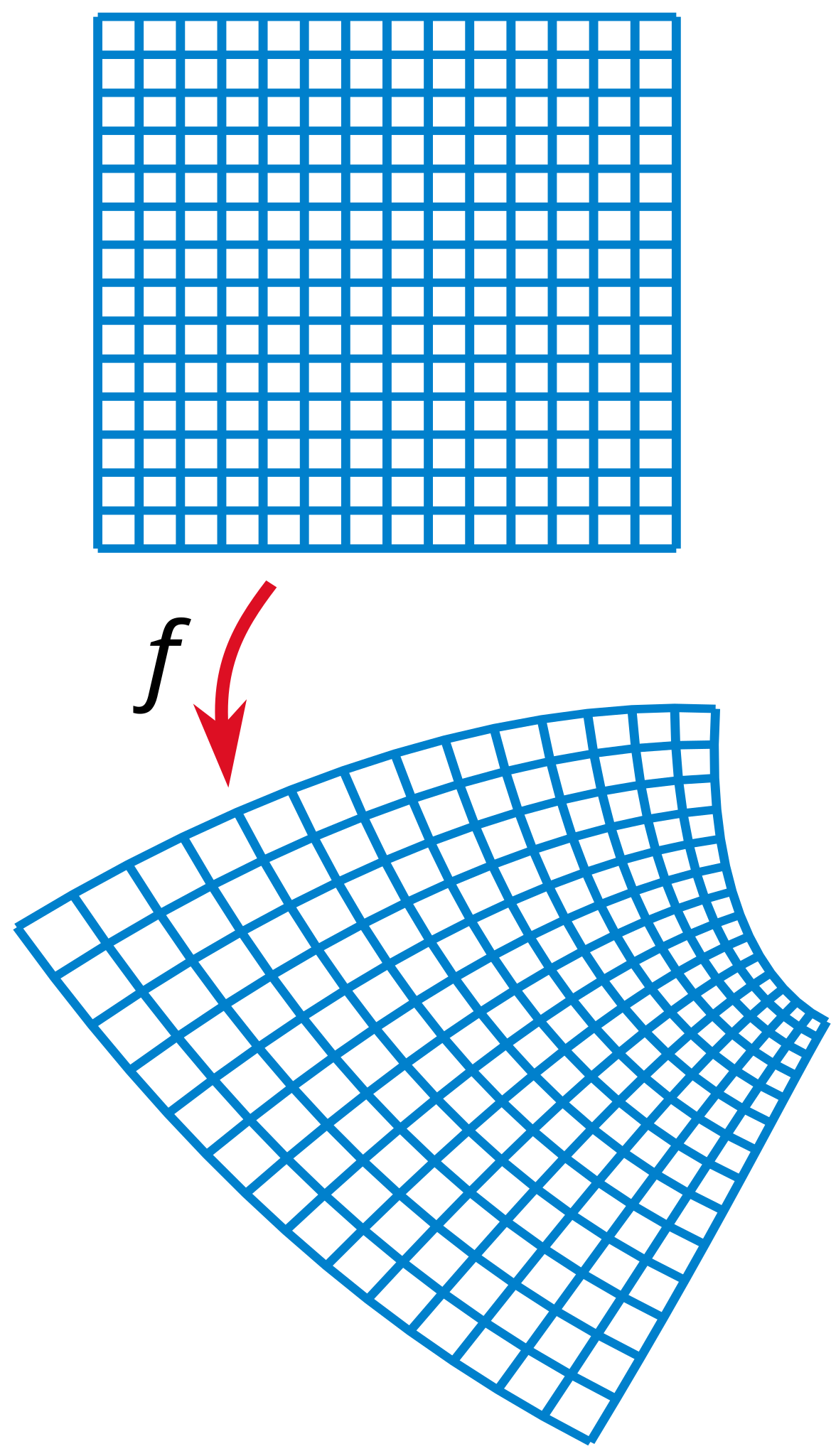
| विवरण | Illustration of a conformal map. |
| दिनांक | |
| स्रोत | self-made with MATLAB, tweaked in Inkscape. |
| लेखक | Oleg Alexandrov |
| SVG genesis | इस वेक्टर चित्र को Inkscape की मदद से बनाया गया था। This file uses translateable embedded text. |
लाइसेंस
| मैं, इस कार्य का/की कॉपीराइट धारक, इस कार्य को सार्वजनिक डोमेन में प्रकाशित करता/करती हूँ। यह पूरे विश्व में लागू होता है। कुछ देशों में यह कानूनी तौर पर नहीं हो सकता है; ऐसा हो तो: मैं सभी को इस कार्य का इस्तेमाल किसी भी उद्देश्य से, बिना किसी बाधाओं के इन शर्तों के कानून द्वारा अनिवार्य किए तक करने की अनुमति देता/देती हूँ। |
Source code (MATLAB)
% Compute the image of a rectangular grid under a a conformal map.

function main()

   N = 15; % num of grid points
   epsilon = 0.1; % displacement for each small diffeomorphism
   num_comp = 10; % number of times the diffeomorphism is composed with itself

   S = linspace(-1, 1, N);

   [X, Y] = meshgrid(S);


   % graphing settings
   lw = 1.0;

   % KSmrq's colors
   red    = [0.867 0.06 0.14];
   blue   = [0, 129, 205]/256;
   green  = [0, 200,  70]/256;
   yellow = [254, 194,   0]/256;
   white = 0.99*[1, 1, 1];

   mycolor = blue;

   % start plotting
   figno=1; figure(figno); clf;

   shiftx = 0; shifty = 0; scale = 1;
   do_plot(X, Y, lw, figno, mycolor, shiftx, shifty, scale)

   I=sqrt(-1);
   Z = X+I*Y;

   % tweak these numbers for a pretty map
   z0 = 1+ 2*I;
   z1 = 0.1+ 0.2*I;
   z2 = 0.2+ 0.3*I;
   a = 0.01;
   b = 0.02;
   shiftx = 0.1; shifty = 1.2; scale = 1.4;
   F = (Z+z0).^2 +a*(Z+z1).^3 +b*(Z+z2).^4;
   F = (1+2*I)*F;

   XF = real(F); YF=imag(F);

   do_plot(XF, YF, lw, figno, mycolor, shiftx, shifty, scale)

   axis ([-1 1.3 -2 2]); axis off;

   saveas(gcf, 'Conformal_map.eps', 'psc2');


function do_plot(X, Y, lw, figno, mycolor, shiftx, shifty, scale)
   figure(figno); hold on;

   [M, N] = size(X);

   X = X - min(min(X));
   Y = Y - min(min(Y));

   a = max(max(max(abs(X))), max(max(abs(Y))));
   X = X/a; Y = Y/a;

   X = scale*(X-shiftx);
   Y = scale*(Y-shifty);

   for i=1:N
      plot(X(:, i), Y(:, i), 'linewidth', lw, 'color', mycolor);
      plot(X(i, :), Y(i, :), 'linewidth', lw, 'color', mycolor);
   end
%   axis([-1-small, 1+small, -1-small, 1+small]);
   axis equal; axis off;
चित्र का इतिहास
फ़ाइलका पुराना अवतरण देखने के लिये दिनांक/समय पर क्लिक करें।
| दिनांक/समय | थंबनेल | आकार | सदस्य | प्रतिक्रिया | |
|---|---|---|---|---|---|
| वर्तमान | 21:51, 27 जनवरी 2008 | | 535 × 937 (34 KB) | Oleg Alexandrov | Make arrow and text smaller |
| 03:36, 23 जनवरी 2008 |  | 535 × 937 (34 KB) | Oleg Alexandrov | {{Information |Description=Illustration of a conformal map. |Source=self-made with MATLAB, tweaked in Inkscape. |~~~~~ |Author= Oleg Alexandrov |Permission= |other_versions= }} {{PD-self}} ==Source code ([[ |
चित्र का उपयोग
निम्नलिखित पन्ने इस चित्र से जुडते हैं :
चित्र का वैश्विक उपयोग
इस चित्र का उपयोग इन दूसरे विकियों में किया जाता है:
- ar.wikipedia.org पर उपयोग
- ba.wikipedia.org पर उपयोग
- ca.wikipedia.org पर उपयोग
- cbk-zam.wikipedia.org पर उपयोग
- cs.wikipedia.org पर उपयोग
- de.wikipedia.org पर उपयोग
- de.wikiversity.org पर उपयोग
- Holomorphie/Kriterien
- Kurs:Riemannsche Flächen (Osnabrück 2022)/Vorlesung 1
- Kurs:Riemannsche Flächen (Osnabrück 2022)/Vorlesung 1/kontrolle
- Satz über die Umkehrabbildung/Implizite Abbildung/C/Zusammenfassung/Textabschnitt
- Kurs:Funktionentheorie (Osnabrück 2023-2024)/Vorlesung 4
- Kurs:Funktionentheorie (Osnabrück 2023-2024)/Vorlesung 4/kontrolle
- el.wikipedia.org पर उपयोग
- en.wikipedia.org पर उपयोग
- es.wikipedia.org पर उपयोग
- fa.wikipedia.org पर उपयोग
- fi.wikipedia.org पर उपयोग
- fr.wikipedia.org पर उपयोग
- gl.wikipedia.org पर उपयोग
- he.wikipedia.org पर उपयोग
- hu.wikipedia.org पर उपयोग
- hy.wikipedia.org पर उपयोग
- id.wikipedia.org पर उपयोग
- it.wikipedia.org पर उपयोग
- ja.wikipedia.org पर उपयोग
इस चित्र के वैश्विक उपयोग की अधिक जानकारी देखें।